Filtering Lorenz-63 With An Ensemble Kalman Filter
In this example, we use the ensemble Kalman filter (EnKF) to filter a partially-observed stochastic Lorenz-63 dynamical system. We compare to the EKF (linearized via Taylor linearization) and a bootstrap particle filter. We observe only the first component \(x_1\) with Gaussian noise, and must infer all three states. This is a difficult but theoretically-tractable task.
The model
We define the classical Lorenz 63 system, and augment it with a small diffusion term, resulting in the SDE:
with the standard chaotic parameters \(\sigma = 10\), \(\rho = 28\), \(\beta = 8/3\). We discretize the drift with Heun's method using a fine inner step size \(\delta t = 0.01\) and assimilate every 35 inner steps (\(\Delta t = 0.35\)). This large assimilation interval makes EKF linearization of the composed multi-step map inaccurate, while the EnKF simply propagates ensemble members through the same nonlinear map without any Jacobian.
Setup and imports
import time

import jax
import jax.numpy as jnp
import matplotlib.pyplot as plt
from jax import jit, random

from cuthbert import filter as run_filter
from cuthbert.enkf import ensemble_kalman_filter
from cuthbert.gaussian import taylor
from cuthbert.gaussian.types import LinearizedKalmanFilterState
from cuthbert.smc import particle_filter
from cuthbertlib.resampling import adaptive, systematic
from cuthbertlib.stats.multivariate_normal import logpdf
from cuthbertlib.types import LogConditionalDensity
Define the Lorenz-63 dynamics
jax.config.update("jax_enable_x64", True)

# Lorenz-63 parameters
lorenz_sigma = 10.0
lorenz_rho = 28.0
lorenz_beta = 8.0 / 3.0

# Discretization and noise
dt_inner = 0.01
n_inner_steps = 35
dt = dt_inner * n_inner_steps
diff_std = 1.0  # Diffusion noise standard deviation
obs_std = 0.3   # Observation noise standard deviation

x_dim = 3
y_dim = 1


def lorenz_drift(x):
    """Lorenz-63 drift function."""
    return jnp.array(
        [
            lorenz_sigma * (x[1] - x[0]),
            x[0] * (lorenz_rho - x[2]) - x[1],
            x[0] * x[1] - lorenz_beta * x[2],
        ]
    )


def lorenz_step(x):
    """Advance one assimilation interval with Heun integration."""

    def body(_, x_curr):
        k1 = lorenz_drift(x_curr)
        x_pred = x_curr + dt_inner * k1
        k2 = lorenz_drift(x_pred)
        return x_curr + 0.5 * dt_inner * (k1 + k2)

    return jax.lax.fori_loop(0, n_inner_steps, body, x)


# Noise covariances
Q = (diff_std**2 * dt) * jnp.eye(x_dim)
chol_Q = jnp.linalg.cholesky(Q)
R = (obs_std**2) * jnp.eye(y_dim)
chol_R = jnp.linalg.cholesky(R)

# Observation model: observe only x_1
H = jnp.array([[1.0, 0.0, 0.0]])
d_obs = jnp.zeros(y_dim)

# Simulate ground truth
num_time_steps = 200
key = random.key(0)

# Spin up to reach the attractor
x = jnp.array([1.0, 1.0, 1.0])
for _ in range(1_000):
    key, dyn_key = random.split(key)
    x = lorenz_step(x) + chol_Q @ random.normal(dyn_key, (x_dim,))

# Initial distribution centered near the attractor
m0 = x
P0 = 2.0 * jnp.eye(x_dim)
chol_P0 = jnp.linalg.cholesky(P0)

# Now simulate with observations
xs, ys = [], []
for t in range(num_time_steps):
    key, dyn_key, obs_key = random.split(key, 3)
    x = lorenz_step(x) + chol_Q @ random.normal(dyn_key, (x_dim,))
    y = H @ x + d_obs + chol_R @ random.normal(obs_key, (y_dim,))
    xs.append(x)
    ys.append(y)

true_states = jnp.stack(xs)
ys = jnp.stack(ys)
times = jnp.arange(num_time_steps) * dt

model_inputs = jnp.arange(num_time_steps + 1)
EKF (Taylor linearization)
We'll use an EKF through the taylor submodule. For this, we need to specify an initial log density, dynamics log-density, observable log-density, and linearization points for each.
def get_init_log_density(model_inputs):
    def init_log_density(x):
        return logpdf(x, m0, chol_P0, nan_support=False)

    return init_log_density, m0


def get_dynamics_log_density(
    state: LinearizedKalmanFilterState, model_inputs
) -> tuple[LogConditionalDensity, jnp.ndarray, jnp.ndarray]:
    lin_point = state.mean

    def dynamics_log_density(x_prev, x):
        return logpdf(x, lorenz_step(x_prev), chol_Q, nan_support=False)

    return dynamics_log_density, lin_point, lorenz_step(lin_point)


def get_observation_func(
    state: LinearizedKalmanFilterState, model_inputs
) -> tuple[LogConditionalDensity, jnp.ndarray, jnp.ndarray]:
    idx = model_inputs - 1

    def obs_log_density(x, y):
        return logpdf(y, H @ x + d_obs, chol_R, nan_support=False)

    return obs_log_density, state.mean, ys[idx]


ekf = taylor.build_filter(
    get_init_log_density,
    get_dynamics_log_density,
    get_observation_func,
    associative=False,
)

jitted_filter = jit(run_filter, static_argnames=["filter_obj"])

n_timing = 20
ekf_states = jitted_filter(ekf, model_inputs)  # warm up
jax.block_until_ready(ekf_states)
_times = []
for _ in range(n_timing):
    _t0 = time.perf_counter()
    jax.block_until_ready(jitted_filter(ekf, model_inputs))
    _times.append(time.perf_counter() - _t0)
ekf_time = float(jnp.median(jnp.array(_times)))

ekf_means = ekf_states.mean
ekf_chol_covs = ekf_states.chol_cov
EnKF
The EnKF propagates an ensemble of particles through the nonlinear dynamics directly. It then performs a Kalman-style update using empirical covariances of these particles. It does not need to compute a Jacobian of the dynamics, unlike the EKF. We need to specify a function that generates initial samples (key, model_inputs) -> x_0, a stochastic dynamics simulator (x, key) -> x_next, and observation parameters.
enkf = ensemble_kalman_filter.build_filter(
    init_sample=lambda key, mi: m0 + chol_P0 @ random.normal(key, m0.shape),
    get_dynamics=lambda mi: lambda x, key: lorenz_step(x)
    + chol_Q @ random.normal(key, (x_dim,)),
    get_observations=lambda mi: (lambda x: H @ x + d_obs, chol_R, ys[mi - 1]),
    n_particles=25,
    inflation=0.05,
    perturbed_obs=True,
)

key, enkf_key = random.split(key)
enkf_states = jitted_filter(enkf, model_inputs, key=enkf_key)  # warm up
jax.block_until_ready(enkf_states)
_times = []
for _ in range(n_timing):
    _t0 = time.perf_counter()
    jax.block_until_ready(jitted_filter(enkf, model_inputs, key=enkf_key))
    _times.append(time.perf_counter() - _t0)
enkf_time = float(jnp.median(jnp.array(_times)))

enkf_means = enkf_states.mean
Bootstrap particle filter
The bootstrap particle filter makes no Gaussian assumption. However, empirically speaking, it requires many more particles than the corresponding EnKF when the EnKF works well. For illustration purposes, we thus use n_filter_particles = 125, i.e., 5x the number of particles used for EnKF.
adaptive_systematic = adaptive.ess_decorator(systematic.resampling, 0.5)

pf = particle_filter.build_filter(
    init_sample=lambda key, mi: m0 + chol_P0 @ random.normal(key, (x_dim,)),
    propagate_sample=lambda key, state, mi: lorenz_step(state)
    + chol_Q @ random.normal(key, (x_dim,)),
    log_potential=lambda s_prev, s, mi: logpdf(
        ys[mi - 1], H @ s + d_obs, chol_R, nan_support=False
    ),
    n_filter_particles=125,
    resampling_fn=adaptive_systematic,
)

key, pf_key = random.split(key)
pf_states = jitted_filter(pf, model_inputs, key=pf_key)  # warm up
jax.block_until_ready(pf_states)
_times = []
for _ in range(n_timing):
    _t0 = time.perf_counter()
    jax.block_until_ready(jitted_filter(pf, model_inputs, key=pf_key))
    _times.append(time.perf_counter() - _t0)
pf_time = float(jnp.median(jnp.array(_times)))

pf_weights = jax.nn.softmax(pf_states.log_weights, axis=-1)
pf_means = jnp.sum(pf_states.particles * pf_weights[..., None], axis=-2)
Compare state estimates
We plot the three state components over time. Remember that only \(x_1\) is observed — the filters must infer \(x_2\) and \(x_3\) from the dynamics alone.
Code to plot state trajectories.
fig, axes = plt.subplots(3, 1, figsize=(12, 8), sharex=True)

dim_labels = ["$x_1$ (observed)", "$x_2$ (unobserved)", "$x_3$ (unobserved)"]

for i, ax in enumerate(axes):
    # True state
    ax.plot(
        times, true_states[:, i], "k-", linewidth=1.0, label="True state", alpha=0.7
    )

    # Observations (only for x_1)
    if i == 0:
        ax.scatter(
            times,
            ys[:, 0],
            s=5,
            color="gray",
            alpha=0.3,
            label="Observations",
            zorder=1,
        )

    # EKF
    ax.plot(
        times,
        ekf_means[1:, i],
        color="#2E86AB",
        linewidth=1.0,
        label="EKF",
        alpha=0.9,
    )

    # EnKF
    ax.plot(
        times,
        enkf_means[1:, i],
        color="#F6AE2D",
        linewidth=1.0,
        label="EnKF",
        alpha=0.9,
    )

    # PF
    ax.plot(
        times,
        pf_means[1:, i],
        color="#F24236",
        linewidth=1.0,
        label="PF",
        alpha=0.8,
    )

    ax.set_ylabel(dim_labels[i], fontsize=12)
    ax.grid(True, alpha=0.2)

axes[0].legend(loc="upper right", fontsize=9, ncol=4)
axes[2].set_xlabel("Time", fontsize=13)
fig.suptitle("Filtered Estimates", fontsize=14)
fig.tight_layout()
fig.savefig("docs/assets/enkf_comparison.png", dpi=150, bbox_inches="tight")
plt.close()
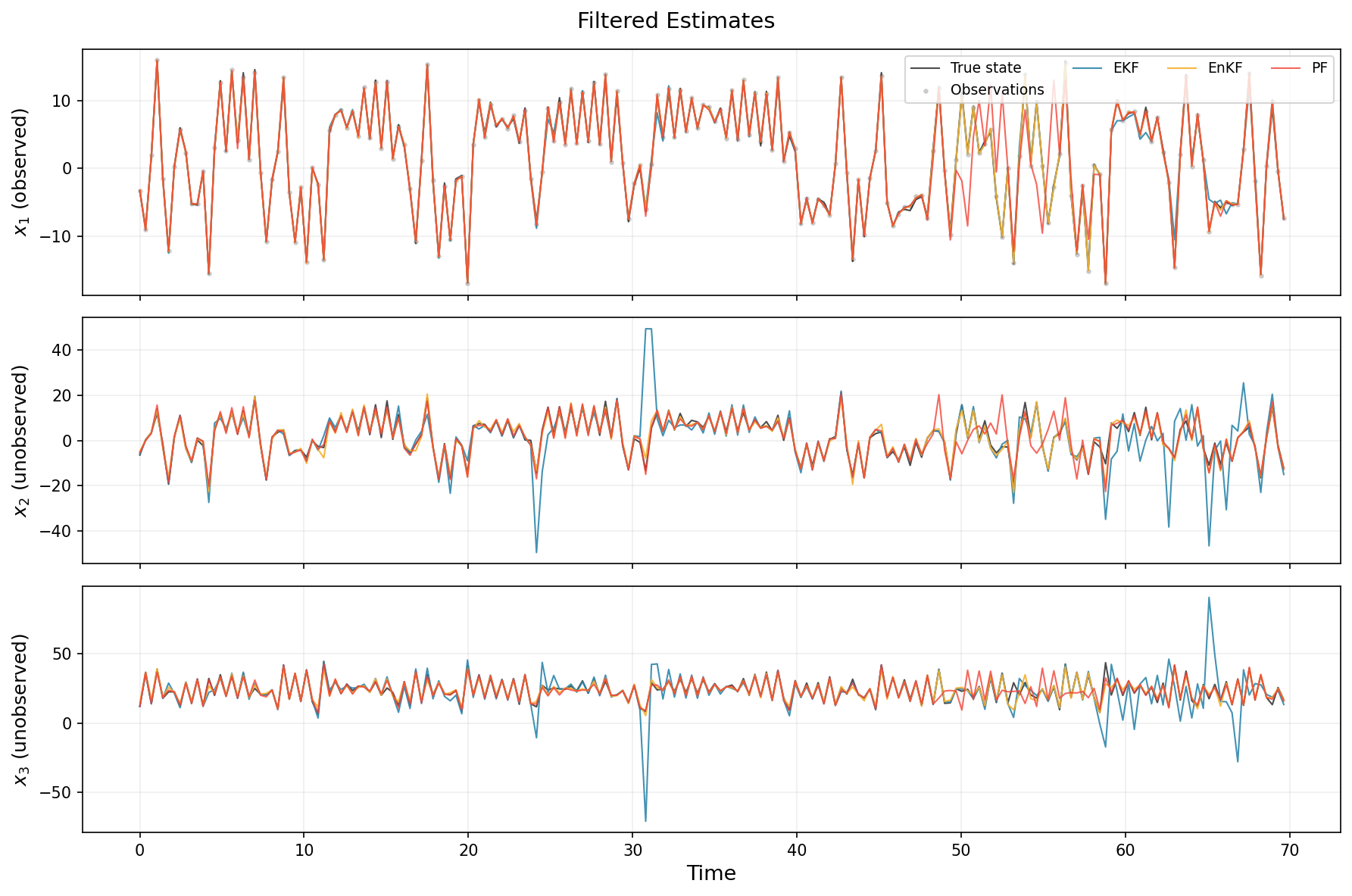
From these results, we can clearly see that the EKF and PF struggled, despite the larger number of particles for the latter. In this example, using ~250 particles would have helped the PF, but with higher computational cost. The EKF would also have performed well given lower observation noise or smaller inter-observation time (and erego less non-linear transitions). The EnKF is the only filter out of the three that does not completely fail at some point.
Metric Comparison
Aside from visual comparisons, we can also compute metrics like RMSE and log-likelihood of the filtered estimates.
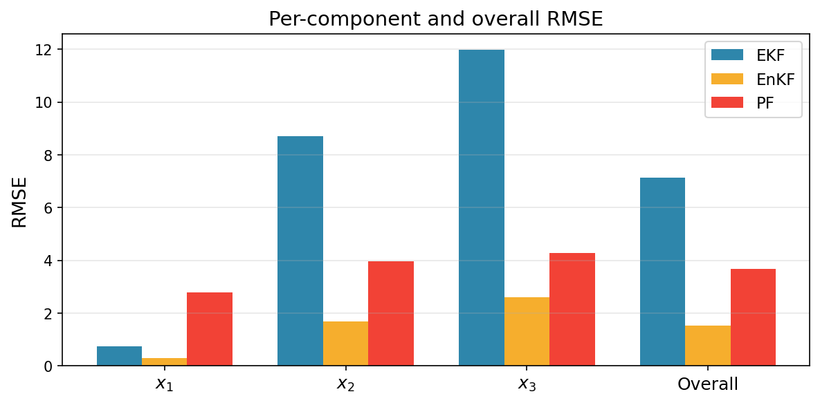
We begin with RMSE of the mean prediction vs. ground truth.
Code to compute and plot RMSE.
def rmse(estimates, truth):
    return jnp.sqrt(jnp.nanmean((estimates - truth) ** 2, axis=0))


ekf_rmses = rmse(ekf_means[1:], true_states)
enkf_rmses = rmse(enkf_means[1:], true_states)
pf_rmses = rmse(pf_means[1:], true_states)

component_names = ["$x_1$", "$x_2$", "$x_3$", "Overall"]
ekf_vals = [*ekf_rmses.tolist(), float(jnp.mean(ekf_rmses))]
enkf_vals = [*enkf_rmses.tolist(), float(jnp.mean(enkf_rmses))]
pf_vals = [*pf_rmses.tolist(), float(jnp.mean(pf_rmses))]

x = jnp.arange(len(component_names))
width = 0.25

fig, ax = plt.subplots(figsize=(8, 4))
ax.bar(x - width, ekf_vals, width, label="EKF", color="#2E86AB")
ax.bar(x, enkf_vals, width, label="EnKF", color="#F6AE2D")
ax.bar(x + width, pf_vals, width, label="PF", color="#F24236")

ax.set_xticks(x)
ax.set_xticklabels(component_names, fontsize=12)
ax.set_ylabel("RMSE", fontsize=13)
ax.set_title("Per-component and overall RMSE", fontsize=14)
ax.legend(fontsize=11)
ax.grid(True, axis="y", alpha=0.3)
fig.tight_layout()
fig.savefig("docs/assets/enkf_comparison_rmse.png", dpi=150, bbox_inches="tight")
plt.close()
The cumulative log-likelihood (log normalizing constant) is a probabilistic estimate of how well each filter predicts the observations.
Code to plot cumulative log-likelihood.
fig, ax = plt.subplots(figsize=(10, 4))

ax.plot(
    times,
    ekf_states.log_normalizing_constant[1:],
    color="#2E86AB",
    linewidth=2,
    label="EKF",
)
ax.plot(
    times,
    enkf_states.log_normalizing_constant[1:],
    color="#F6AE2D",
    linewidth=2,
    label="EnKF",
)
ax.plot(
    times,
    pf_states.log_normalizing_constant[1:],
    color="#F24236",
    linewidth=2,
    label="PF",
)

ax.set_xlabel("Time", fontsize=13)
ax.set_ylabel("Cumulative log-likelihood", fontsize=13)
ax.set_ylim(bottom=float(ekf_states.log_normalizing_constant[1:].min()) * 1.05, top=0.0)
ax.legend(fontsize=11)
ax.grid(True, alpha=0.2)
fig.tight_layout()
fig.savefig("docs/assets/enkf_comparison_loglik.png", dpi=150, bbox_inches="tight")
plt.close()

print(f"Final log-likelihood — EKF:  {ekf_states.log_normalizing_constant[-1]:.2f}")
print(f"Final log-likelihood — EnKF: {enkf_states.log_normalizing_constant[-1]:.2f}")
print(f"Final log-likelihood — PF:   {pf_states.log_normalizing_constant[-1]:.2f}")
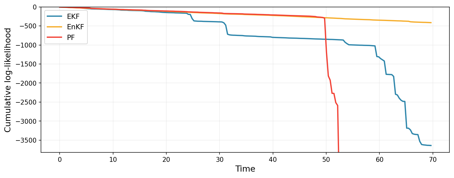
In both metrics, the EKF and PF completely collapse in performance at some point, whilst EnKF maintains good state estimates. Once again, this example is somewhat cherry-picked, in that small modifications to the data-generating process would have resulted in strong performance from the EKF or PF, but illustrates the robustness of the EnKF.
Runtime comparison
One benefit of the EnKF is its ability to handle nonlinear dynamics with relatively low computational cost. Indeed, the EKF must compute a Jacobian at every time point, and the PF typically relies on a large number of particles to maintain accuracy. Let us compare the time it took to run each filter (not counting time to JIT).
Code to plot runtime comparison.
fig, ax = plt.subplots(figsize=(6, 4))

filter_names = ["EKF", "EnKF", "PF"]
run_times = [ekf_time, enkf_time, pf_time]
colors = ["#2E86AB", "#F6AE2D", "#F24236"]

ax.bar(filter_names, run_times, color=colors)
ax.set_ylabel("Wall-clock time (s)", fontsize=13)
ax.set_title(f"Filter runtime (median over {n_timing} runs, excl. JIT)", fontsize=14)
ax.grid(True, axis="y", alpha=0.3)
fig.tight_layout()
fig.savefig("docs/assets/enkf_comparison_timing.png", dpi=150, bbox_inches="tight")
plt.close()
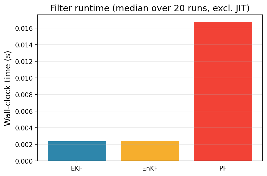
Under the settings that we used, the EnKF has comparable computational demand to the EKF, and is significantly cheaper than the PF.
Key Takeaways
- Lorenz-63 with a large assimilation interval (\(\Delta t = 0.35\)) is a regime where the EKF breaks down: the linearization of the 35-step composed map is highly inaccurate near the attractor's saddle points.
- EnKF handles this naturally — each ensemble member is propagated through the same nonlinear multi-step integrator, with no Jacobian required. The ensemble covariances capture the true non-Gaussian predictive uncertainty.
- Particle filter makes no Gaussian assumption but can suffer at large \(\Delta t\) without more particle: the bootstrap proposal is the dynamics prior which becomes broad relative to the likelihood at long intervals.
- Unified API benefit: switching between EKF, EnKF, and PF only changes the filter construction — the simulation, observation, and plotting code is shared.
Next Steps
- Play With
dt: Shrinkn_inner_stepstoward 1–2 steps to see the EKF recover as linearization becomes accurate again, or raise it further and see EKF completely collapse. - Play With Particles: Increase
n_filter_particlesfor the particle filter and see the PF avoid collapse across a longer time horizon. - Parameter learning: Use
jax.gradthrough the EnKF's differentiable log-likelihood to learn Lorenz-63 parameters (\(\sigma\), \(\rho\), \(\beta\)) from data. - More examples: Check out the other examples.